class: title-slide # R for Paleolimnology ## PALS 2018 Workshop ### W. Brent Thorne¹ & Dewey W. Dunnington² .footnote[¹Department of Earth Sciences, Brock University, St. Catharines, ON, Canada L2S 3A1; bthorne2@brocku.ca ²Department of Earth and Environmental Science, Acadia University, Wolfville, NS, Canada B4P 2R5; ] --- background-image: url(https://funnytimes.com/wp-content/uploads/1995/10/199510043.jpg) background-position: 95% 95% class: big # What You Will Learn -- 1. What is R and what is RStudio? -- 2. How do I get my data into R? -- 3. How to structure and transform your data -- 4. How to visualize your paleolimnological data --- # Getting Started Install **[R](https://cran.r-project.org/)** and **[RStudio](https://rstudio.com/)** onto your machince. -- - *Feel free to ask for help!* -- ### Success! <img src="https://www.w-t-w.org/en/wp-content/uploads/2014/02/Studying-Computer-Programming.jpg" width=200 align="middle"> .footnote[Please follow allong using the online resource we have built which can be found [here](https://paleolimbot.github.io/r4paleolim/).] --- # Tutorial 1 .black[Basic R] 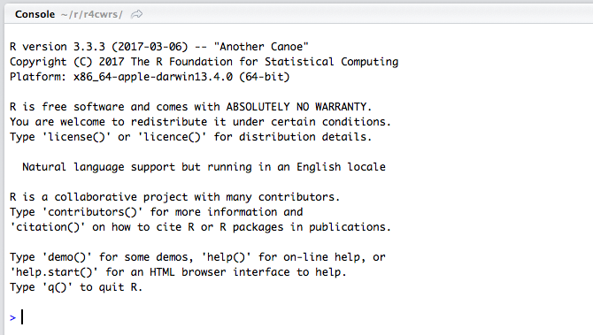 --- ## Prerequisites -- We will be using the <a href="https://www.tidyverse.org/" target="_blank"><img src="https://www.tidyverse.org/images/hex-tidyverse.png" width="100" align="middle"></a> package: -- ```r install.packages("tidyverse") library(tidyverse) ``` -- ### Easy Right! --- ## Expressions -- ```r 1 + 1 ``` ``` ## [1] 2 ``` -- ```r 2 * 5 ``` ``` ## [1] 10 ``` -- ```r 2 * (5 + 1) ``` ``` ## [1] 12 ``` --- ## Variables -- ```r x <- 1 + 1 ``` -- ```r x ``` ``` ## [1] 2 ``` -- ```r x + 2 ``` ``` ## [1] 4 ``` --- ## Character Vectors ```r mytext <- "I am text" mytext ``` ``` ## [1] "I am text" ``` --- ## Functions An argument with an input which returns an output value. -- Let's calculate a square root: ```r sqrt(4) ``` ``` ## [1] 2 ``` -- Find the largest number in a list: ```r max(2, 6, 7, 2, 10) ``` ``` ## [1] 10 ``` --- ## Keyword Arguments ```r paste("string1", "string2", sep = "_") ``` ``` ## [1] "string1_string2" ``` --- background-image: url(https://pics.me.me/it-doesnt-work-why-it-works-why-2349750.png) --- ## Functions (Help) Use the `?` to call the help documentation to any function in R! ```r ?paste ``` --- ## Functions (Help) **Description** Concatenate vectors after converting to character. **Usage** ``` paste (..., sep = " ", collapse = NULL) paste0(..., collapse = NULL) ``` **Arguments** <table><tr valign="top"><td><code>...</code></td><td><p>one or more <span style="font-family: Courier New, Courier; color: #666666;"><b>R</b></span> objects, to be converted to character vectors.</p></td></tr><tr valign="top"><td><code>sep</code></td><td><p>a character string to separate the terms. Not <code><a href="NA.html">NA_character_</a></code>.</p></td></tr><tr valign="top"><td><code>collapse</code></td><td><p>an optional character string to separate the results. Not <code><a href="NA.html">NA_character_</a></code>.</p></td></tr></table> --- ## Vectors -- Combine sets of numbers: ```r myvector <- c(10, 9, 8, 7, 2) myvector ``` ``` ## [1] 10 9 8 7 2 ``` -- Or do it with sets of characters: ```r mytextvector <- c("word1", "word2", "word3") mytextvector ``` ``` ## [1] "word1" "word2" "word3" ``` -- ```r myothervector <- 13:16 myothervector ``` ``` ## [1] 13 14 15 16 ``` --- ## Vectors ```r start <- 25 end <- start + 5 start:end ``` ``` ## [1] 25 26 27 28 29 30 ``` --- ## Indexing - What's inside our vector? -- ```r myvector <- c(10, 9, 8, 7, 2) myvector[1] ``` ``` ## [1] 10 ``` -- ```r myvector[5] ``` ``` ## [1] 2 ``` --- ## Indexing - Indexing with a **vector**. -- ```r myvector[1:3] ``` ``` ## [1] 10 9 8 ``` -- This is equivalent to: ```r myvector[c(1, 2, 3)] ``` ``` ## [1] 10 9 8 ``` --- ## Indexing ### TRUE/FALSE -- ```r myvector[myvector > 7] ``` ``` ## [1] 10 9 8 ``` -- ```r myvector > 7 ``` ``` ## [1] TRUE TRUE TRUE FALSE FALSE ``` --- ## Missing Values Missing values are represented in R using `NA`, or "not assigned". -- ```r mean(c(NA, 1, 2, 3)) ``` ``` ## [1] NA ``` -- Use the **argument** `na.rm = TRUE` to remoe `NA` values. ```r mean(c(NA, 1, 2, 3), na.rm = TRUE) ``` ``` ## [1] 2 ``` --- ## Data Frames The vast majority of data in R is kept in a **tibble** (often called a **data frame**), which is a collection of **vectors** of the same length. You can think of a **tibble** as a table, with each column in the table being of the same type (numeric, character, TRUE/FALSE, etc.). -- ```r my_tibble <- tibble( number = c(1, 2, 3), name = c("one", "two", "three"), is_one = c(TRUE, FALSE, FALSE) ) my_tibble ``` ``` ## # A tibble: 3 x 3 ## number name is_one ## <dbl> <chr> <lgl> ## 1 1 one TRUE ## 2 2 two FALSE ## 3 3 three FALSE ``` --- ## Data Frames You can get these values as vectors again using the `$` operator, which allows you to extract a vector from a data frame. -- ```r my_tibble$number ``` ``` ## [1] 1 2 3 ``` ```r my_tibble$name ``` ``` ## [1] "one" "two" "three" ``` ```r my_tibble$is_one ``` ``` ## [1] TRUE FALSE FALSE ``` --- ## Loading Packages Base R functionality is designed to provide basic functions to help with data analysis, but may add-ons are available and code you find online (including here, shortly) will often tell you to load a "package" using `library()`. -- ```r library(packagename) ``` -- The `tidyverse` package actually installs and loads a family of useful packages for us, a list of which we can access using `tidyverse_packages()`. Try it! ```r tidyverse_packages() ``` ``` ## [1] "broom" "cli" "crayon" "dplyr" "dbplyr" ## [6] "forcats" "ggplot2" "haven" "hms" "httr" ## [11] "jsonlite" "lubridate" "magrittr" "modelr" "purrr" ## [16] "readr" "readxl\n(>=" "reprex" "rlang" "rstudioapi" ## [21] "rvest" "stringr" "tibble" "tidyr" "xml2" ## [26] "tidyverse" ``` --- ## Loading Packages If a packge you wish to use is not able to be loaded using `library()` it just means you nead to install it onto your computer first! ```r install.packages("tidyverse") ``` --- ## Script Editor In reality, very little of the code you type will be directly in the prompt. Instead, you will use RStudio's script editor to run commands so that you can go back and edit them or run them from the beginning.  --- ## Environment Use the **Environment** tab in RStudio to see which variables you have already assigned. 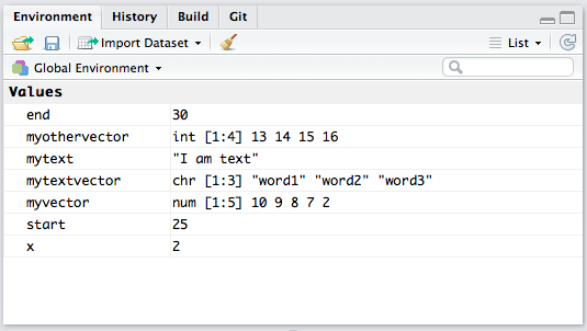 --- # Tutorial 2 .black[Working with Tables using the Tidyverse] - In this tutorial we will use the tidyverse to manipulate and summarise tabular data. --- ## Read in the Data Let's bring in the data provided by Dewey Dunnington! ```r halifax_geochem <- read_csv( "http://paleolimbot.github.io/r4paleolim/data/halifax_geochem.csv", col_types = cols(.default = col_guess()) ) ``` --- ## Read in the Data - The data contains several bulk geochemical parameters from a recent study of Halifax drinking water reservoirs¹, including Pockwock Lake, Lake Major, Bennery Lake, Lake Fletcher, Lake Lemont, First Chain Lake, First Lake, and Second Lake. (Later, we will take a look at the core locations as well as the geochemical data). .footnote[ [1] Dunnington, Dewey W., I. S. Spooner, Wendy H. Krkošek, Graham A. Gagnon, R. Jack Cornett, Chris E. White, Benjamin Misiuk, and Drake Tymstra. 2018. “Anthropogenic Activity in the Halifax Region, Nova Scotia, Canada, as Recorded by Bulk Geochemistry of Lake Sediments.” [https://doi.org/10.1080/10402381.2018.1461715](https://doi.org/10.1080/10402381.2018.1461715) ] --- ## Viewing a Data Frame The variable we have just created (halifax_geochem) is a tibble, which is a table of values much like you would find in a spreadsheet (you will notice that we loaded it directly from an Excel spreadhseet). -- ```r View(halifax_geochem) # will display a graphic table browser ``` ```r glimpse(halifax_geochem) # will display a text summary of the object ``` ``` ## Observations: 326 ## Variables: 9 ## $ core_id <chr> "BEN15-2", "BEN15-2", "BEN15-2", "BEN15-2", "BEN... ## $ depth_cm <dbl> 0.0, 0.5, 1.0, 1.5, 2.0, 2.5, 3.0, 3.5, 4.0, 4.5... ## $ age_ad <dbl> 2015.903, 2015.188, 2014.474, 2012.950, 2011.425... ## $ C_percent <dbl> 14.75718, 14.65701, 14.94983, 14.54558, 14.40408... ## $ `C/N` <dbl> 12.15765, 12.17829, 11.92338, 11.67900, 11.61200... ## $ d13C_permille <dbl> -30.24752, -30.31042, -30.35799, -30.33835, -30.... ## $ d15N_permille <dbl> 2.461962, 2.447662, 2.336219, 2.528572, 2.662515... ## $ K_percent <dbl> 1.0026000, 1.0857000, 0.9782000, 0.9423000, 1.07... ## $ Ti_percent <dbl> 0.1693000, 0.1823000, 0.1678000, 0.1664000, 0.18... ``` ```r head(halifax_geochem) # will display the first few rows of the data ``` ``` ## # A tibble: 6 x 9 ## core_id depth_cm age_ad C_percent `C/N` d13C_permille d15N_permille ## <chr> <dbl> <dbl> <dbl> <dbl> <dbl> <dbl> ## 1 BEN15-2 0 2016. 14.8 12.2 -30.2 2.46 ## 2 BEN15-2 0.5 2015. 14.7 12.2 -30.3 2.45 ## 3 BEN15-2 1 2014. 14.9 11.9 -30.4 2.34 ## 4 BEN15-2 1.5 2013. 14.5 11.7 -30.3 2.53 ## 5 BEN15-2 2 2011. 14.4 11.6 -30.4 2.66 ## 6 BEN15-2 2.5 2010. 14.4 11.9 -30.3 2.48 ## # ... with 2 more variables: K_percent <dbl>, Ti_percent <dbl> ``` --- ## Selecting Columns - One way to subset `halifax_geochem` is to subset by column, for which we will use the `select()` function. -- We may only be interested in the stable isotope information, represented by the columns `d13C_permille` and `d15N_permille`. ```r stable_isotope_data <- select( halifax_geochem, core_id, depth_cm, age_ad, d13C_permille, d15N_permille ) ``` --- ## Select Columns - The first argument to the `select()` function is the original data frame (in this case, `halifax_geochem`), and the remaining arguments are the names of the columns to be selected. -- To select the `core_id`, `age_ad`, `Ti`, and `K` columns, you would use the following R command: ```r geochem_data <- select(halifax_geochem, core_id, depth_cm, age_ad, Ti_percent, K_percent) ``` --- ## Select Columns - Some column names in `halifax_geochem` contain characters that could be interpreted as an operation (e.g., `C/N`, which is the name of the column and not `C` divided by `N`). -- - To select these columns, you will need to surround the column name in backticks: ```r select(halifax_geochem, core_id, depth_cm, age_ad, `C/N`) ``` --- ## Select Columns ### Exercises - Use `View()`, `glimpse()`, and `head()` to preview the two data frames we just created. Do they have the columns you would expect? - Use `select()` to select `core_id`, `depth_cm`, C/N, d13C, and d15N, and assign it to the variable `cn_data`. -- --- ## Filtering Rows - Another way to subset `halifax_geochem` is by filtering rows using column values, similar to the filter feature in Microsoft Excel. - This is done using the `filter()` function. For example, we may only be interested in the core from Pockwock Lake. ```r pockwock_data <- filter(halifax_geochem, core_id == "POC15-2") ``` -- - Passing multiple conditions means each row must satisfy all of the conditions, such that to obtain the data from core POC15-2 where the depth in the core was 0 cm, we can use the following call to `filter()`: ```r pockwock_surface_data <- filter(halifax_geochem, core_id == "POC15-2", depth_cm == 0) ``` --- ## Filtering Rows - It is very important that there are two equals signs within `filter()`! - Other operators are: `<=`, `>=`, `<`, `>`, or `%in%` ```r data_recent <- filter(halifax_geochem, age_ad >= 1950) ``` -- We could also find observations from multiple cores: ```r pockwock_major_data <- filter(halifax_geochem, core_id %in% c("POC15-2", "MAJ15-1")) ``` --- ## Filtering Rows ### Exercises - Use `View()`, `glimpse()`, and `head()` to preview the data frames we just created. Do they have the rows you would expect? - Use `filter()` to find observations from the core FCL16-1 with an age between 1900 and present, and assign it to a name of your choosing. - Are there any observations with a C/N value greater than 20? (hint: you will have to surround `C/N` in backticks) -- --- ## Selecting and Filtering - Often we need to use both `select()` and `filter()` to obtain the desired subset of a data frame. - To do this, we need to pass the result of `select()` to `filter()`, or the result of `filter()` to `select()`. -- Let's create a data frame of recent (age greater than 1950) stable isotope measurements (you'll recall that we selected stable isotope columns in the data frame `stable_isotope_data`): ```r recent_stable_isotopes <- filter(stable_isotope_data, age_ad >= 1950) recent_stable_isotopes2 <- select( data_recent, core_id, depth_cm, age_ad, d13C_permille, d15N_permille ) ``` --- ## Selecting and Filtering ### Exersices - Use `View()`, `glimpse()`, and/or `head()` to verify that `recent_stable_isotopes` and `recent_stable_isotopes_2` are identical. --- ## The Pipe (%>%) Instead of creating intermediary variables every time we want to subset a data frame using `select()` and `filter()`, we can use the pipe operator (`%>%`) to pass the result of one function call to another. -- ```r recent_stable_isotopes_pipe <- halifax_geochem %>% filter(age_ad >= 1950) %>% select(core_id, depth_cm, age_ad, d13C_permille, d15N_permille) ``` ## The Pipe (%>%) ### Exerscises - Inspect `recent_stable_isotopes_pipe` to ensure it is identical to `recent_stable_isotopes`. - Create a data frame of stable isotope data from surface samples (`depth_cm == 0`) using `halifax_geochem`, `filter()`, `select()`, and `%>%` and assign it to a variable of a suitable name. -- --- ## Arranging (sorting) A Data Frame - Sometimes it is desirable to view rows in a particular order, which can be used to quickly determine min and max values of various parameters. This is done using the `arrange()` function. For example, it may make sense to view `halifax_geochem` in ascending `core_id` and `depth_cm` order (most recent first): -- ```r halifax_geochem %>% arrange(core_id, depth_cm) ``` ``` ## # A tibble: 326 x 9 ## core_id depth_cm age_ad C_percent `C/N` d13C_permille d15N_permille ## <chr> <dbl> <dbl> <dbl> <dbl> <dbl> <dbl> ## 1 BEN15-2 0 2016. 14.8 12.2 -30.2 2.46 ## 2 BEN15-2 0.5 2015. 14.7 12.2 -30.3 2.45 ## 3 BEN15-2 1 2014. 14.9 11.9 -30.4 2.34 ## 4 BEN15-2 1.5 2013. 14.5 11.7 -30.3 2.53 ## 5 BEN15-2 2 2011. 14.4 11.6 -30.4 2.66 ## 6 BEN15-2 2.5 2010. 14.4 11.9 -30.3 2.48 ## 7 BEN15-2 3 2008. 14.4 11.9 -30.3 2.53 ## 8 BEN15-2 3.5 2005. 14.3 12.0 -30.2 2.60 ## 9 BEN15-2 4 2002. 14.0 12.0 -30.2 2.60 ## 10 BEN15-2 4.5 1999. 13.7 12.1 -30.2 2.48 ## # ... with 316 more rows, and 2 more variables: K_percent <dbl>, ## # Ti_percent <dbl> ``` --- ## Arranging (sorting) A Data Frame - Or descending depth order (most recent last): ```r halifax_geochem %>% arrange(core_id, desc(depth_cm)) ``` ``` ## # A tibble: 326 x 9 ## core_id depth_cm age_ad C_percent `C/N` d13C_permille d15N_permille ## <chr> <dbl> <dbl> <dbl> <dbl> <dbl> <dbl> ## 1 BEN15-2 29 1742. 14.5 13.4 -29.3 3.54 ## 2 BEN15-2 28 1751. 14.5 13.5 -29.3 3.60 ## 3 BEN15-2 27 1759. 15.1 13.4 -29.4 3.60 ## 4 BEN15-2 26 1768. 15.9 13.5 -29.5 3.57 ## 5 BEN15-2 25 1776. 16.7 13.4 -29.6 3.42 ## 6 BEN15-2 24 1784. 16.8 13.4 -29.5 3.42 ## 7 BEN15-2 23 1793. 16.5 13.5 -29.4 3.39 ## 8 BEN15-2 22 1801. 17.2 13.4 -29.4 3.41 ## 9 BEN15-2 21 1810. 17.3 13.6 -29.4 3.22 ## 10 BEN15-2 20 1818. 17.6 13.5 -29.4 3.18 ## # ... with 316 more rows, and 2 more variables: K_percent <dbl>, ## # Ti_percent <dbl> ``` --- ## Distinct Values It is often useful to know which values exist in a data frame. For example, I've told you that the core locations are for various lakes in the halifax area, but what are they actually called in the dataset? To do this, we can use the `distinct()` function. ```r halifax_geochem %>% distinct(core_id) ``` ``` ## # A tibble: 8 x 1 ## core_id ## <chr> ## 1 BEN15-2 ## 2 FCL16-1 ## 3 FLE16-1 ## 4 FLK12-1 ## 5 LEM16-1 ## 6 MAJ15-1 ## 7 POC15-2 ## 8 SLK13-1 ``` - The `distinct()` function can take any number of column names as arguments, although in this particular dataset there isn't a good example for this. --- ## Calculating columns using `mutate()` - To create a brand-new column, we can use the `mutate()` function. This creates a column in a way that we can use existing column names to calculate a new column. For example, we could convert the `age_ad` column to years before 1950: ```r halifax_geochem %>% mutate(age_bp = 1950 - age_ad) %>% select(core_id, age_ad, age_bp) ``` ``` ## # A tibble: 326 x 3 ## core_id age_ad age_bp ## <chr> <dbl> <dbl> ## 1 BEN15-2 2016. -65.9 ## 2 BEN15-2 2015. -65.2 ## 3 BEN15-2 2014. -64.5 ## 4 BEN15-2 2013. -62.9 ## 5 BEN15-2 2011. -61.4 ## 6 BEN15-2 2010. -59.6 ## 7 BEN15-2 2008. -57.8 ## 8 BEN15-2 2005. -54.9 ## 9 BEN15-2 2002. -52.1 ## 10 BEN15-2 1999. -49.3 ## # ... with 316 more rows ``` -- - Or, we could convert the `K_percent` and `Ti_percent` columns to parts per million: ```r halifax_geochem %>% mutate( K_ppm = K_percent * 10000, Ti_ppm = Ti_percent * 10000 ) %>% select(core_id, K_percent, K_ppm, Ti_percent, Ti_ppm) ``` ``` ## # A tibble: 326 x 5 ## core_id K_percent K_ppm Ti_percent Ti_ppm ## <chr> <dbl> <dbl> <dbl> <dbl> ## 1 BEN15-2 1.00 10026 0.169 1693 ## 2 BEN15-2 1.09 10857. 0.182 1823 ## 3 BEN15-2 0.978 9782 0.168 1678 ## 4 BEN15-2 0.942 9423 0.166 1664 ## 5 BEN15-2 1.08 10784. 0.183 1832. ## 6 BEN15-2 1.09 10863 0.183 1830 ## 7 BEN15-2 1.04 10374. 0.176 1762 ## 8 BEN15-2 0.97 9700 0.167 1670 ## 9 BEN15-2 1.12 11175 0.179 1791 ## 10 BEN15-2 1.01 10064. 0.17 1700. ## # ... with 316 more rows ``` --- ## Summarising A Data Frame So far we have looked at subsets of `halifax_geochem`, but what if we want per-core averages instead of raw data values? Using the tidyverse, we can `group_by()` the `core_id` column, and `summarise()`: ```r halifax_geochem %>% group_by(core_id) %>% summarise(mean_CN = mean(`C/N`)) ``` ``` ## # A tibble: 8 x 2 ## core_id mean_CN ## <chr> <dbl> ## 1 BEN15-2 12.8 ## 2 FCL16-1 14.2 ## 3 FLE16-1 12.4 ## 4 FLK12-1 12.8 ## 5 LEM16-1 12.6 ## 6 MAJ15-1 NA ## 7 POC15-2 NA ## 8 SLK13-1 NA ``` --- ## Summarising A Data Frame Here `group_by()` gets a list of columns, for which each unique combination of values will get one row in the output. `summarise()` gets a list of expressions that are evaluated for every unique combination of values defined by `group_by()` (e.g., `mean_CN` is the `mean()` of the `C/N` column for each core). Often, we want to include a number of summary columns in the output, which we can do by pasing more expressions to `summarise()`: ```r halifax_geochem %>% group_by(core_id) %>% summarise( mean_CN = mean(`C/N`), min_CN = min(`C/N`), max_CN = max(`C/N`), sd_CN = sd(`C/N`) ) ``` ``` ## # A tibble: 8 x 5 ## core_id mean_CN min_CN max_CN sd_CN ## <chr> <dbl> <dbl> <dbl> <dbl> ## 1 BEN15-2 12.8 11.6 13.6 0.648 ## 2 FCL16-1 14.2 12.1 16.5 1.05 ## 3 FLE16-1 12.4 10.5 13.3 0.830 ## 4 FLK12-1 12.8 10.6 14.9 1.02 ## 5 LEM16-1 12.6 11.8 13.1 0.307 ## 6 MAJ15-1 NA NA NA NA ## 7 POC15-2 NA NA NA NA ## 8 SLK13-1 NA NA NA NA ``` --- ## Summarising A Data Frame You will notice that in for several cores the summary values are `NA`, or missing. This is because R propogates missing values unless you explicitly tell it not to. To fix this, you could replace ``mean(`C/N`)`` with ``mean(`C/N`, na.rm = TRUE)``. Other useful functions to use inside `summarise()` include `mean()`, `median()`, `sd()`, `sum()`, `min()`, and `max()`. These all take a vector of values and produce a single aggregate value suitable for use in `summarise()`. One special function, `n()`, you can use (with no arguments) inside `summarise()` to tell you how many observations were aggregated to produce the values in that row. ```r halifax_geochem %>% group_by(core_id) %>% summarise( mean_CN = mean(`C/N`, na.rm = TRUE), min_CN = min(`C/N`, na.rm = TRUE), max_CN = max(`C/N`, na.rm = TRUE), sd_CN = sd(`C/N`, na.rm = TRUE), n = n() ) ``` ``` ## # A tibble: 8 x 6 ## core_id mean_CN min_CN max_CN sd_CN n ## <chr> <dbl> <dbl> <dbl> <dbl> <int> ## 1 BEN15-2 12.8 11.6 13.6 0.648 35 ## 2 FCL16-1 14.2 12.1 16.5 1.05 49 ## 3 FLE16-1 12.4 10.5 13.3 0.830 37 ## 4 FLK12-1 12.8 10.6 14.9 1.02 33 ## 5 LEM16-1 12.6 11.8 13.1 0.307 35 ## 6 MAJ15-1 15.7 14.3 18.4 1.09 51 ## 7 POC15-2 15.2 13.6 17.4 1.26 52 ## 8 SLK13-1 11.4 10.3 11.9 0.443 34 ``` --- ## Summarising A Data Frame ### Exerscises - Assign the data frame we just created to a variable, and inspect it using View() and str(). Which cores have the most terrestrial C/N signature? Which cores have the most aquatic signature? - Create a similar data frame to the one we just created but using C_percent. Which cores had the highest peak organic value. - Which cores had the oldest estimated basal date? --- # Tutorial 3 <<<<<<< HEAD ## Prerequisites test ======= ## Creating Visualizations using ggplot <img src='https://d33wubrfki0l68.cloudfront.net/0ab849ed51b0b866ef6895c253d3899f4926d397/dbf0f/images/hex-ggplot2.png' class='center' width='200'> --- ## Creating Visualizations using ggplot ### Prerequisites >>>>>>> 6d0fca143b60ed8bc8e9296fc9b1626271f7d243